Le tadalafil possède une affinité marquée pour la PDE5, mais épargne en grande partie les isoformes PDE1, PDE2 et PDE11, réduisant ainsi le risque d’effets extra-caverneux. L’action se traduit par une augmentation contrôlée de la circulation sanguine locale, indépendante des variations alimentaires. Sa pharmacocinétique repose sur une absorption digestive rapide, un métabolisme hépatique par CYP3A4 et une distribution tissulaire large. La biodisponibilité reste stable, et l’équilibre plasmatique est atteint en quelques jours lors d’administrations répétées. Les interactions cliniquement significatives surviennent avec les inhibiteurs puissants de CYP3A4 tels que le kétoconazole. Dans la littérature pharmacologique, acheter cialis 20 mg est souvent associé à des schémas d’utilisation basés sur la durée prolongée de son action.
Untitled
Particle Size Analysis by Laser Diffraction Introduction
3. The scattering pattern at the detectors is the
The underlying assumption in the design of laser
sum of the individual scattering patterns
diffraction instruments is that the scattered light
pattern formed at the detector is a summation of
the scattering pattern produced by each particle
Experimental
that is being sampled. Deconvolution of the
Prior to analysis, the dispersion cell is filled with
resultant pattern generates information about the
clean, deionised water and left to allow thermal
scattering pattern produced by each particle and,
equilibrium to take place. The instrument
upon inversion, information about the size of the
automatically aligns so that the incident path of
the laser is aligned with the optical arrays. The
cleanliness of the system is then checked, and a background is taken. By comparing the signal intensity of the system without a sample present, to the intensity with a sample, the obscuration of the laser beam may be calculated, giving some idea of the material concentration in the dispersal cell. Too high a concentration results in multiple scattering, too low and the signal strength is inadequate to register at the detectors. Figure 2 below illustrates a comparison between the signals obtained from an empty system (red), with that from a particle sample (green). The background signal should always be lower than your sample signal!
Data Graph - Light Scattering
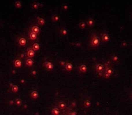
Figure 1: Light scattering patterns observed for
In essence, each particle scatter pattern is
1 3 5 7 9 12 15 18 21 24 27 30 33 36 39 42 45 48 51
comprehensive mathematical solution to the
scattering of incident light by spherical particles;
Figure 2: Background and sample scattering data
the Mie Theory. This theory indicates the
necessity for a precise knowledge of the real and
Suitable dispersion procedures should be followed
imaginary components of the refractive index of
to ensure that the powder is dispersed and
the material being analysed, to determine particle
minimum agglomeration has taken place. Care
size and particle size distribution. When a good fit
must also be taken to ensure that the dispersal
is obtained, then we know all of the relevant
cell contains no air bubbles or that particle
information in order to deconvolute the Mie
fracture is not occurring as the instrument is not
pattern into meaningful particle size information.
capable of distinguishing between agglomerates,
All laser diffraction instruments rely on three basic
1. The particles scattering the light are spherical in
Sonification is an option to aid particle dispersion
although again, care must be taken to ensure the
2. There is little to no interaction between the light
correct intensity and duration of sonification to
avoid primary particle breakage. The particle size distribution will depend on the optical model used to calculate it! The real and
AN003 Particle size analysis by laser diffraction rev 0.doc
Data Graph - Light Scattering
imaginary components of the refractive index are
a vital part of the particle characterisation
equation. In the case of an unknown particle
refractive index (if a literature value is
unavailable), the optical properties may be
derived by varying the input values and comparing
the resultant scatter pattern with the measured
Imaginary part of refractive index = 0.1, 20 February 2004 15:32:21
Data Graph - Light Scattering
In figure 3 below, we see the difference the
imaginary part of the refractive index makes to the
resulting size distribution. The question is which
Fit data(weighted)Imaginary part of refractive index = 1.0, 20 February 2004 15:32:21
We clearly see the evolution in scatter pattern as
the actual data starts to approach the theoretical,
until at an imaginary RI component of 1, the
patterns coincide. At this point, we can say that
this scatter pattern is the most correct, and in this
Imaginary part of refractive index = 0.01
case, the true size distribution will be the blue line
Imaginary part of refractive index = 0.1 Imaginary part of refractive index = 1.0
Figure 3: Size distributions using varying
Conclusions
If we look at the theoretical scatter pattern
2. Laser diffraction particle sizing requires both
compared with the measured data, we get an
the real and imaginary components of the
instant idea of the goodness of fit. Figures 4, 5
and 6 illustrate the comparison when using an
3. By adjusting RI values manually, the scatter
imaginary refractive index of 0.01. 0.1 and 1.0
pattern may be manipulated until actual and
theoretical are congruent. At this point, we
may say our input RI is correct, and the
Data Graph - Light Scattering
resultant size distribution is representative of
Imaginary part of refractive index = 0.01, 20 February 2004 15:32:21
Escubed Ltd
AN003 Particle size analysis by laser diffraction rev 0.doc
ABSTRACTS OF PRESENTATIONS AT SCIENTIFIC MEETINGS 1. Woolley, Dorothy E., and Paola S. Timiras. Effects of sex hormones on electroshock seizure threshold and on glycogen and electrolyte distribution in brain of rats. The Pharmacologist 1(2):66, 1959. Timiras, Paola S., and Dorothy E. Woolley. Effects of estradiol on brain excitability in male rats. Proceedings of the First International Congress
⊲ accommodates a nondifferentiable, non-⊲ with (mixed) continuous or discrete state⊲ using a locally linear value function⊲ Entry and exit from industry, technol-• Use sequential importance sampling (parti-⊲ to integrate unobserved variables out of⊲ to estimate ex-post trajectory of unob-⊲ Stationary distribution of MCMC chain⊲ Because we prove the computed likeli-⊲ Ef

 Particle Size Analysis by Laser Diffraction